By MohammadHossein Jamshidi, Ph.D student of Physics/Cosmology at Shahid Beheshti University, Iran.
I’m a Ph.D student of Physics/Cosmology at Shahid Beheshti University. I have also been an animation engineer in the game industry since 2012. You may find some of my works on my GitHub.
Here I share some of the ideas and techniques of using Blender during my research in cosmology. Although these are specifically used in cosmology, I am confident that similar ideas apply to other areas of science. All the files shown here are available for free on this GitHub repository.
What is Cosmology and what do I do?
Cosmology is the science of studying the physical world on gigantic scales, both in size and time; so large that a galaxy could be considered as a single point, and so long that a millennium could be taken as just one frame of time!
My interest in the world of cosmology lies in Cosmic Microwave Background (CMB) radiation, the light rays that reach us from the very early universe. The CMB has a temperature of about 2.7 Kelvin (around -270 degrees Celsius) and is nearly uniform across the sky; however, it has some tiny fluctuations (of size 10 to 10 K) across the sky which contain very fascinating information from the early definable times, and also the history of the universe. These light rays are quite the last things that we can observe in the sky, coming from the farthest distance that could ever be observed. They have recorded numerous events in the history of the universe, and now we are fortunate enough to be able to decode some of their interesting information.
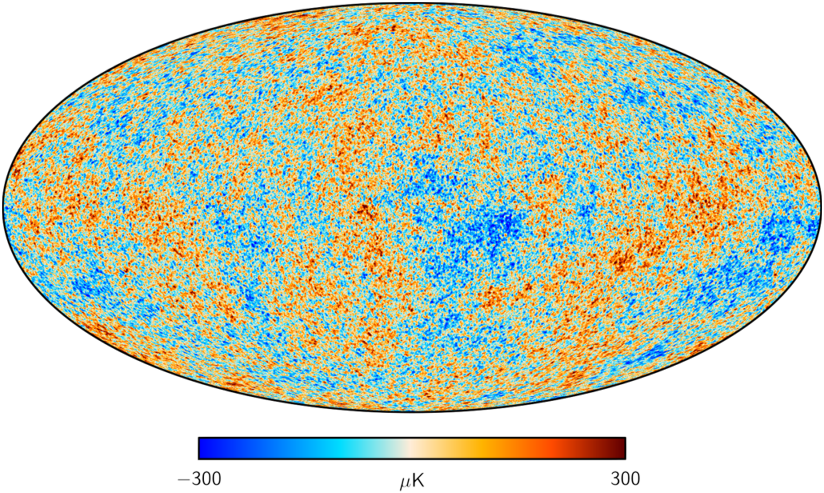
Credit: ESA and the Planck Collaboration
Inspirations to use Geo Nodes for Cosmology
The early ideas to use Blender for Cosmology were enlightened in my mind from the creative and delightful works of Seanterelle on YouTube. I was impressed by his nice simulations with Geo Nodes that had eye-catching performance, and I tried to use Geometry Nodes for cosmological computations.
In 2024, for one of our projects on the CMB, we utilized Geometry Nodes as a tool for computation, visualization, and algorithm debugging. We needed a tool to visualize caps and stripes of different sizes on the CMB sky, to check how much of their areas overlap with the Galactic Mask (the areas where we can’t receive CMB light due to contamination by our Galaxy). By utilizing the Geo Nodes and some simple rigging, we were able to make such a visualizer.
One may access the results of that project in this paper. This visualization served as a starting point for us to use Geo Nodes in broader areas and more use cases.
Geometry Nodes for Computation
Geometry Nodes compute things on mesh elements in parallel. If the mesh elements (faces or vertices, etc.) are considered “data storage slots” and “processing threads”, we can perfectly utilize Geo Nodes for doing “Single Instruction Multiple Data” (SIMD) computations. Although other tools, such as CUDA or Compute shaders might be faster, Geo Nodes provides also a free debugger and visualizer. It is especially perfect for small-scale projects; we can calculate and visualize instantly, and in most cases, we can reach the final numerical result in real-time.
Sometimes we just need a fast and reliable tool, especially for tests on our calculation procedure, to check whether its results are physically correct. Geo Nodes is a handy tool to test the correctness of a procedure/algorithm on a smaller scale. In the following sections, we’ll see some examples of real-life cosmology that we could utilize Geo Nodes not only for visualization and debugging, but also for computation.
Cosmology with Geometry Nodes
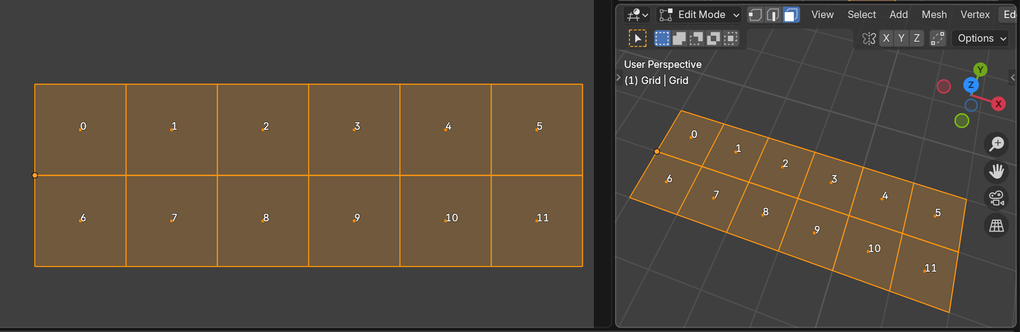
As pointed out in the previous section, to work with Geometry Nodes for manipulating data, we need a 3D mesh to store the data on and perform processes with. Making proper meshes for our data is the first step towards utilizing Geo Nodes.
How are the sky maps stored?
From a computational perspective, it is decisive how to store the data appropriately. The way we store the data can drastically decrease the amount of calculations.
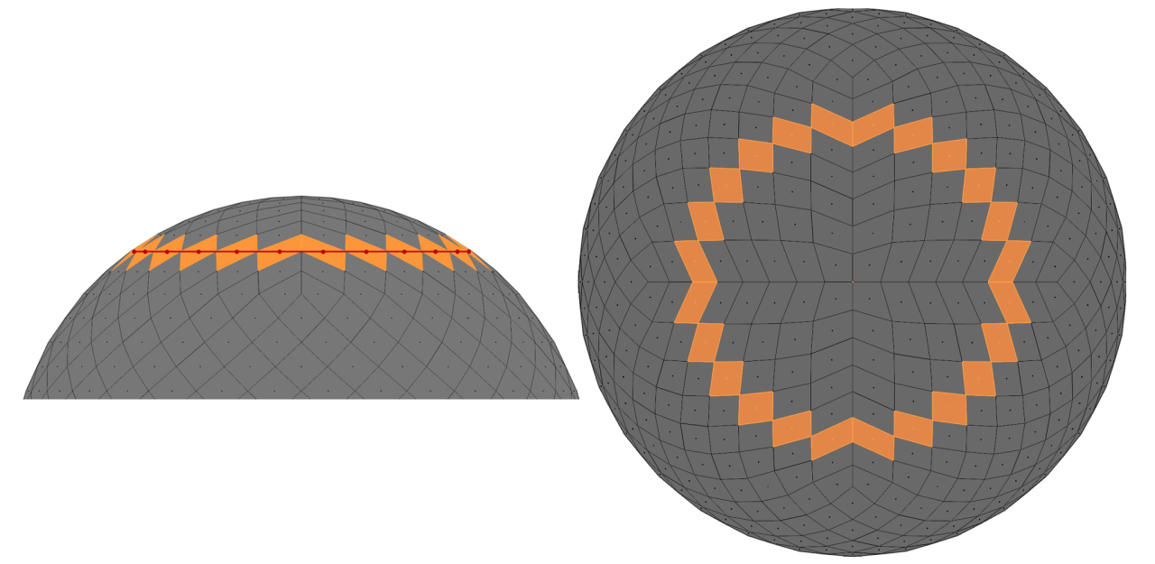
Cosmologists and geologists need to work with spherical maps/data, and they must store their data in a way that enables faster spherical calculations. There is a special kind of pixelation of the sphere called HEALPix (Hierarchical Equal Area isoLatitude Pixelation).
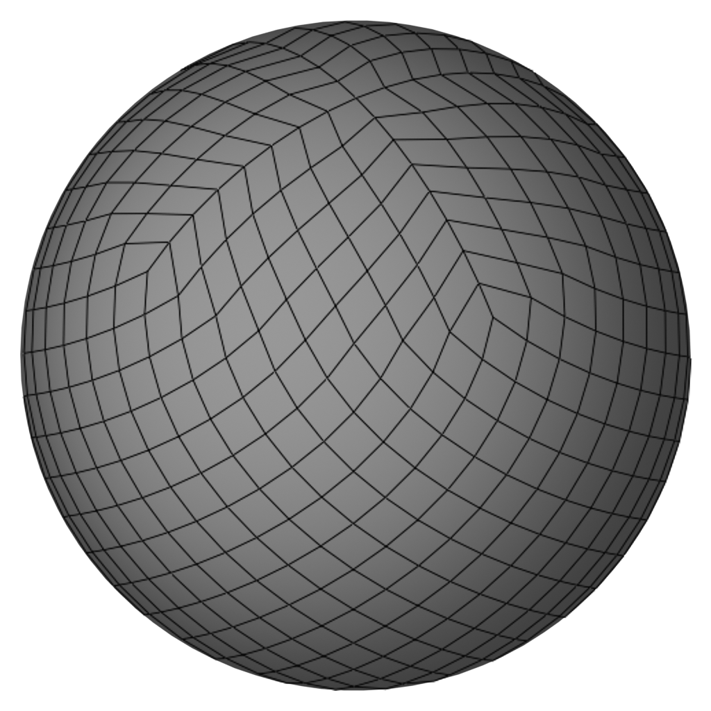
As suggested by its name, the pixels of this pixelation have the same area. This sphere can be partitioned into rings of pixels that are parallel to the equator. None of its pixel centers are located at the poles (dealing with poles is problematic most of the time). This pixelation is great for storing the data, and doing spherical math with it is very efficient.
To make a HEALPix sphere at different resolutions, you can find a step-by-step tutorial here.
Despite the benefits of HEALPix pixelation, working with the positioning and ordering(numbering/indices) of these pixels can sometimes be complicated. In the following, we’ll see how Geo Nodes saves us from tedious stuff in map analysis.
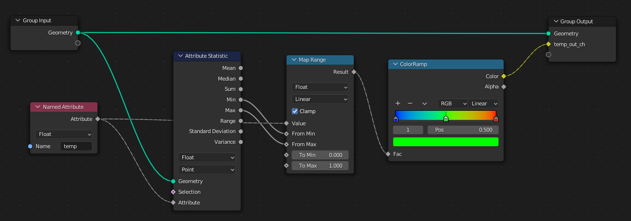
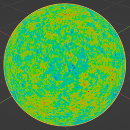
Visualization of CMB sky using Geo Nodes
Once we create a HEALPix sphere with proper pixel ordering, we can use face attributes of the HEALPix mesh to store the CMB data and visualize it using Geo Nodes. A detailed tutorial for visualizing CMB maps is available here, though I briefly describe the steps here. First, we need to inject the map data (e.g., temperature of the CMB) into the mesh and store the data of each pixel on each face of the HEALPix sphere. Now we should take the min and max temperature, and put them in the range as colors.
Projection makes life easier
Geometry Nodes’ data(attribute) projection is a very powerful tool that is beneficial in many real-life examples. In this section, I’ll bring a few.
Pixel-preserving map rotation
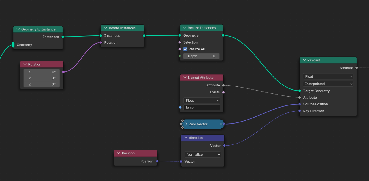
In processing spherical data in cosmology, we need map transformations, and it is valuable mathematically and computationally to keep the HEALPix pixelation during these transformations. Here, we see how it is possible to rotate a map and preserve the pixelation. It may seem hard to perform such a task, but it would be very easy with the attribute projection tool in Geometry Nodes.
The idea is to rotate the HEALPix mesh (the one that contains the map on its faces) and project its data to another HEALPix sphere that is not rotated (transformed). This is actually the idea behind all the map transformations discussed in this section.
Implement-wise, in Geo Nodes, we need to:
- Make a virtual copy of the original sphere;
- Rotate it;
- Cast a ray from inside the sphere towards each pixel and see at which pixel it collides;
- Project the ray casted attribute on the original mesh.
Following these steps, one will have a nice rotated map, while the pixelation is kept intact:
Doppler boost addition / removal
Map rotation is not the only use case of the attribute projection; another case that we found useful is to distort a map while keeping the pixelation. The idea is very similar to the one for rotation, that of projecting a distorted map onto an undistorted sphere.
Different physical processes may lead to a distortion in the map. For instance, the Doppler effect is a physical phenomenon that causes the CMB map to be changed by several means, and one of them is aberration (a special kind of distortion). If we weren’t moving with respect to the light sources, the light rays coming to us would be received in the commonly expected directions. However, as our planet (and galaxy) moves in space (with respect to light sources), we receive the incoming light rays in changed directions (see the video below). This phenomenon is called aberration. This happens to all the light rays (including CMB) coming to us, so every sky map will be distorted because of our motion with respect to the light sources.
The aberration effect can be easily simulated in Geometry Nodes. If we know at which speed we are moving and in which direction, we can compute the aberrated direction of the incoming light rays (we estimate it by the change in the frequency of the observed light rays). To simulate the aberration, we need to distort pixel borders (vertices of the HEALPix sphere). If we calculate the aberrated direction of each vertex, we will end up with a distorted sphere. Now, if we project this distorted sphere onto a normal HEALPix sphere, we will end up with the aberrated map of the CMB in HEALPix pixelation.
Another effect that occurs when we move across the sky is the Doppler boost effect, which is the change in the wavelengths of the incoming light rays because of our motion with respect to the sources. Each CMB light ray will also be affected by this motion, and so we measure a different temperature for it. Knowing how the temperature changes regarding our velocity, we can compute the change in each pixel. Mixing the aberration and the Doppler boost, we can simulate our motion in the sky with Geo Nodes:
Capturing images from sky map
In one cosmology project, we needed to investigate some anomalous spots in the CMB sky map by machine learning. For the machine to have similar-looking data from the sky, we needed square images of various regions of the sky. The confusing indexing of the HEALPix maps was misleading for us at first. After a while, we found that by using the Geo Nodes’ attribute projection, we could cleanly prepare our desired images without overthinking about the confusing indexing of HEALPix.
The idea is the same. Place a square plane at where you want to capture the image, and apply the projection in the same way as the previous parts, and you will finish with nice square images from the CMB map.
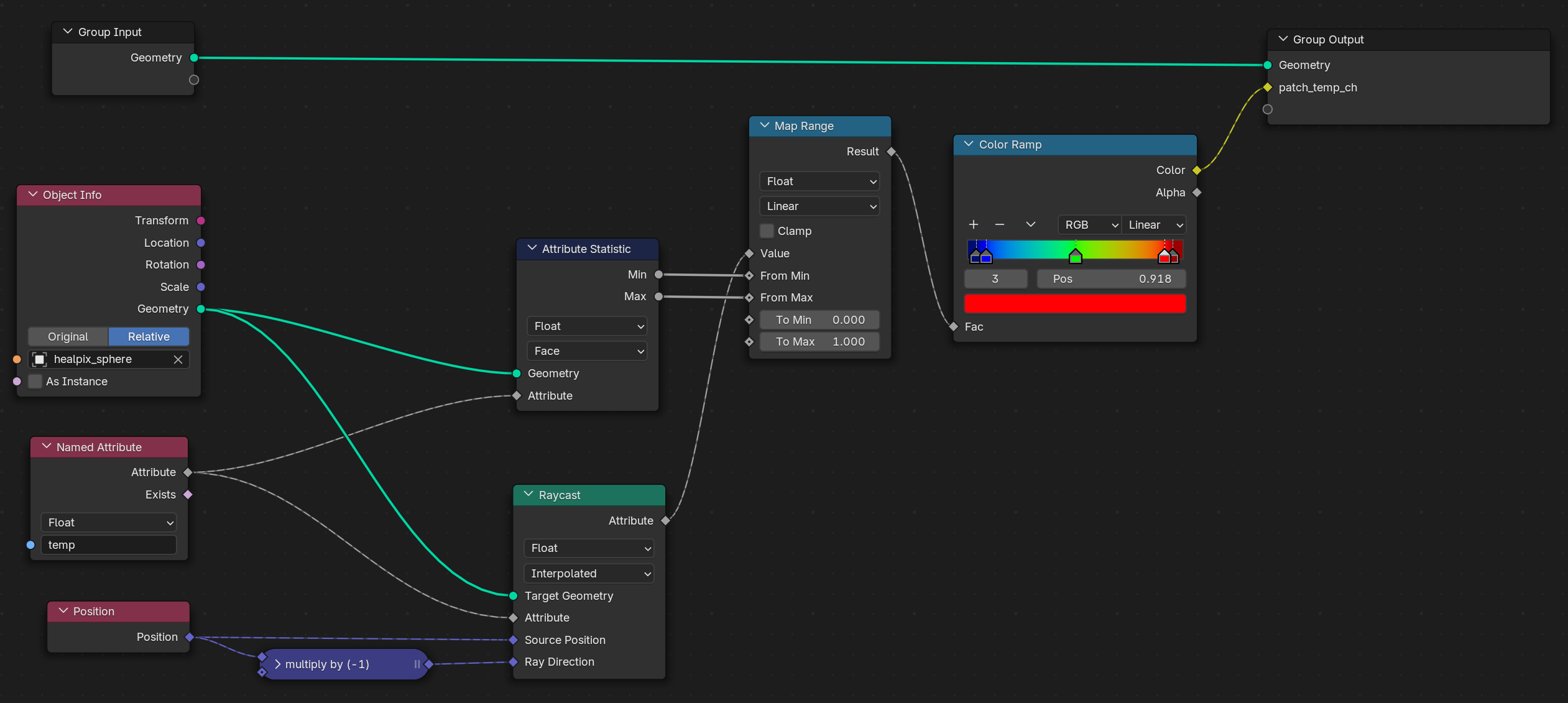
We can either store the indices or the temperature directly, but for technical reasons, I preferred pixel indices. Then I spanned the whole sky by placing the plane on top of each area and storing the pixel indices underneath it. So this way, we had the proper dataset for our machine learning program.
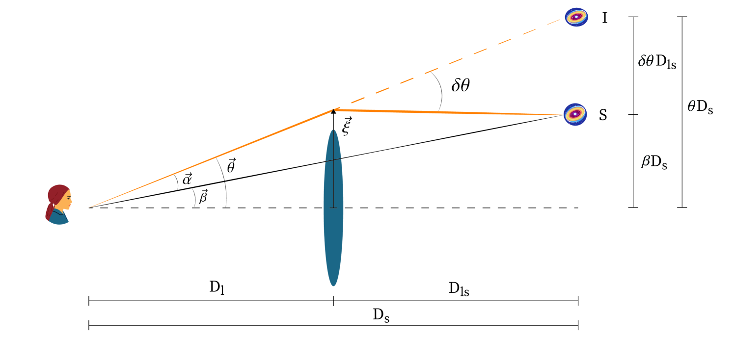
Gravitational lensing in real time!
Massive objects in the sky cause the light rays to be bent in their path. When we observe a galaxy, if a massive object is in our line of sight, we see a deformed image of it. From our perspective, sources of light are deflected and differ from their original locations (just as an ordinary optical lens causes us to see objects deformed or dislocated). If the mass of the bending object is not too large, the lensing would be weak. This form of lensing is easy to calculate and is more common in the CMB.
Prat, J., & Bacon, D. “Weak Gravitational Lensing.” arXiv preprint arXiv:2501.07938 (2025).
To simulate the weak lensing, we need to find the deflected location of the light sources after lensing. To calculate this in Blender, one can consider each vertex of a mesh as a point source of light and manipulate its location by the deflection angle
( is the mass of the massive object and is the perpendicular distance from the massive object). In the video below, you see the lensed image of Suzanne; it is assumed as a light source, being affected by a massive object.
To utilize it in a real-world scenario, one can take an image of a galaxy and put it on a plane (with enough vertex count) and do the same thing with its vertices to simulate the lensing on the galaxy image:
Image from ESA/Hubble & NASA
This is very helpful for preparing samples to train a machine to find sources of lensing or delensing an image.
Sky sphere unwrapped! (Mollweide view)
To visualize spherical maps on a 2D plane, there is a common style in which the whole sky is flattened into a 2D image. There are many such interesting mappings; each has its use case. Cosmologists commonly use a mapping called Mollweide.
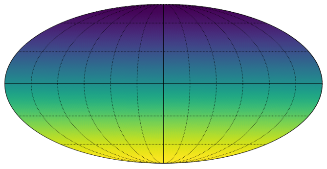
There are packages available that help us to plot in Mollweide view, but they have their own limitations. Geo Nodes enable us to implement these 3 to 2D mappings and allow us to do almost anything to our plots. For example, we can visualize the changes on the map in real-time or draw customized contours.
To plot in Mollweide, first, we need to cut the sphere to unwrap it (a cut in one meridian). We work with the HEALPix sphere, which has a special topology. First, we should add some edges to complete an edge loop on the meridian we want to cut, and then split(cut) it so the sphere can be unwrapped.
Then, to project points with the Mollweide method, we need to iterate for one coordinate, and we need a for loop in Geo Nodes to do this.
Once we split the mesh and find the projected locations, our sphere will be mapped to Mollweide.
Mollweide in Blender, when combined with other pixelation-preserving techniques in other sections, will provide a real-time Mollweide visualizer. For example, in the following video, you see the map rotation combined with the Mollweide projection:
Computation on pixels in parallel
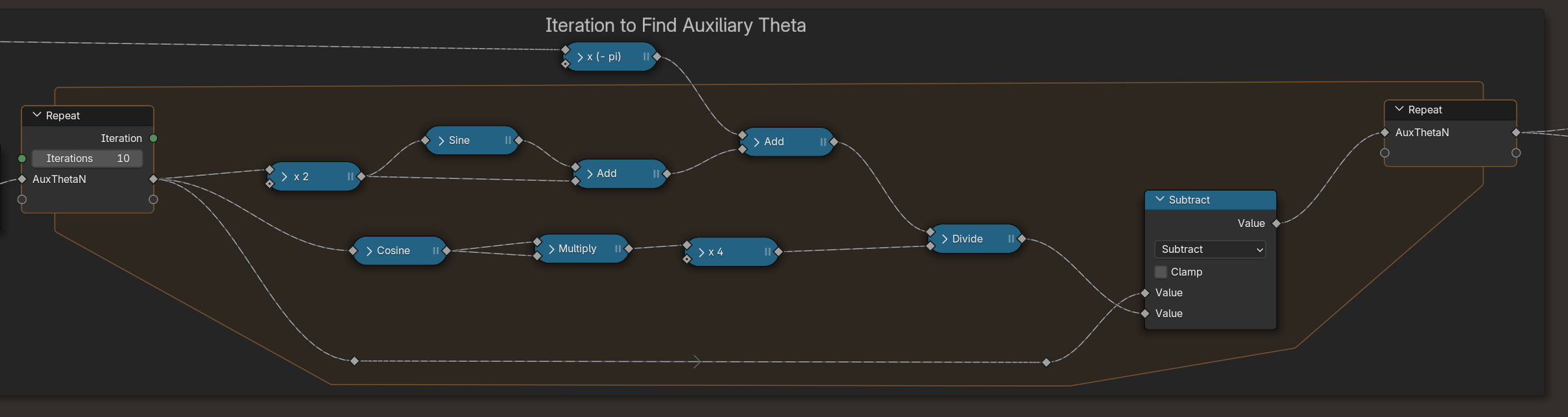
As mentioned earlier, one can utilize Geometry Nodes to compute things in parallel. Calculating things on each pixel of a spherical map is a very vital use case. In cosmology, it is very common to describe a spherical map/image using spherical harmonic functions (or spherical harmonics). Spherical harmonics are like Fourier series, but they live on the surface of a sphere. They help us to separate large and small features of spherical maps to investigate their physical origins.
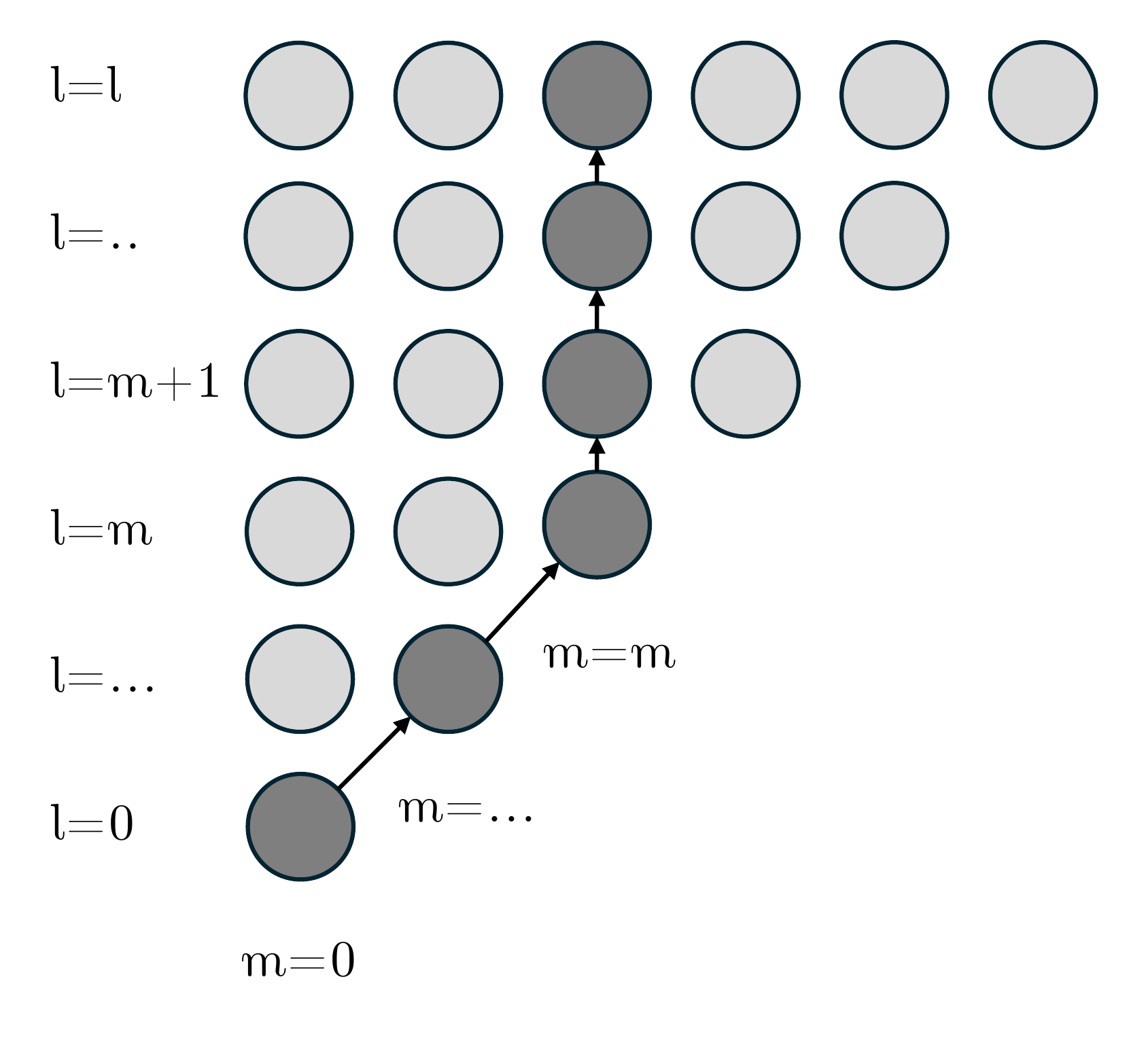
Spherical harmonics are typically shown by . They are functions of direction (θ,ϕ) and have two indices and . In our case, a direction is represented by a pixel on the HEAPix sphere (or a face of its mesh). Computing spherical harmonics in general is a bit tricky because they should be calculated using recursive mathematical relations (or they will overflow very quickly using direct formulas). There are several ways to create a recursive relation that gives us the spherical harmonics, but most of them are not numerically stable. They will overflow or get zero very quickly. The image below shows the path to calculate the spherical harmonics stably using recursive relations.
Having a stable recursive relation, we should implement the formula using nodes. Writing long mathematical formulas in Geo Nodes is quite cumbersome, and I think it requires a script node to handle such scenarios more easily; however, the final results are very nice, fast, and handy.
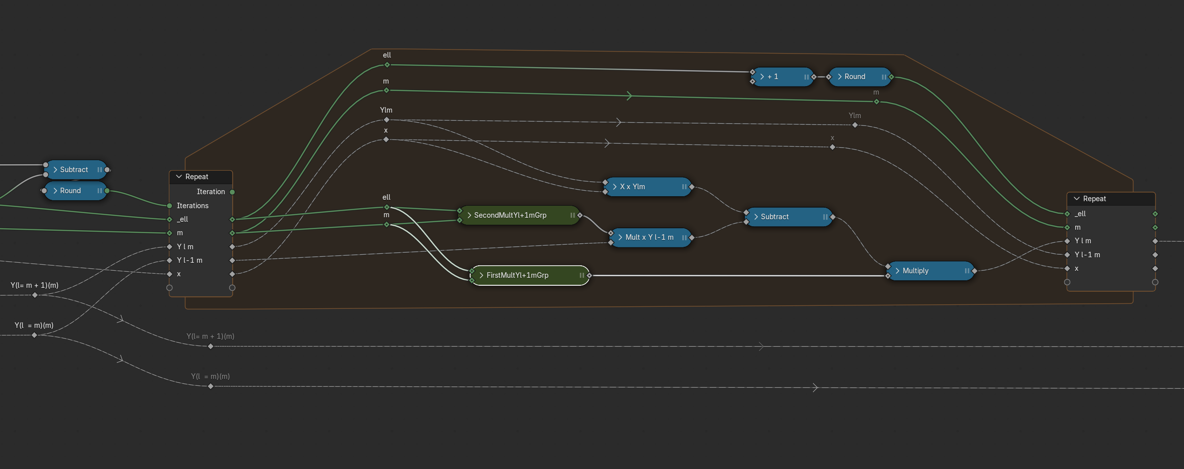
Once we implement the formula correctly, it can be shown on the surface of the sphere just like a map:
Float32? No problem with doing precision cosmology
As we know, Geometry Nodes use float32 numbers, which are not precise enough for analysing high-resolution maps or sky partitions, and we need float64 numbers. However, it is not an endpoint to use Geo Nodes for precise computations. It is possible to emulate float64 numbers and their operations with two float32 numbers. There are a lot of algorithms out there for emulating 64-bit numbers with two float32s. The only change that should be made in our process for Geometry Nodes is to store the 64-bit number in two float channels, which means either by using two separate channels or by using a vector channel that holds the two parts of the actual number. One can create custom functions to mimic the operators of the separated numbers. To visualize, though, it would be enough to convert the number back to a float32 and visualize it.
Other areas of physics
From the first time I saw the nice works of Seanterelle on YouTube, to when I was developing the above techniques, and so far, I have been thinking about “what other areas of physics can make use of Geometry Nodes?”. I’m confident that physicists in other areas can utilize Geo Nodes in their field. I can imagine using it for simulating crystals, spin systems, astrophysical systems, liquids, protein folding, general relativity calculations/visualizations, and many-body systems. The list definitely doesn’t end here. You can also think about the use cases and develop simulations in your field.
Acknowledgement
I would like to express my sincere gratitude to Professor Nima Khosravi for his invaluable guidance in the scientific aspects of these works.
A special thanks to Dr.Abdolali Banihshemi for his collaboration throughout both the project and the writing of this post.
I’m also grateful to Francesco Siddi, Fiona Cohen, and Dr. Sybren Stüvel for their kind support to publish this user story.